Time Series: Digging into the ARIMA Model

What is a time series exactly?

Time series are simply data represented over some period of time, where each variable is that point in time. One of the more clearer examples being stock prices over a certain interval such as every minute or every day, the infamous Black Friday every year, anything represented as a sequence of data in chronological order. What makes time series analysis useful is the idea that it can take underlying data and provide expectations of what future data will look like. When working with this type of data, we can break it down into 4 components:

Trend: the longer term directional move
Seasonality: patterns that occur at fixed intervals
Cyclicality: recurring rises/falls that do not occur at fixed intervals
Error/Shocks: random fluctuations and unexpected events

There are also 3 major tasks we must do when working with time series data:

Filtering: using past and present data to estimate the current state and reduce noise
Smoothing: estimating historical states
Forecasting: "predicting" future values based on historical patterns, producing an expectation

The reason for emphasizing the quotes with the word prediction is that when working with time series in the context of predicting a stock price we have to keep in mind that this assumes that we are expecting, based on the data, the status quo to continue into the future without having some type of regime change in markets that will cause our time series forecast to be wildly inaccurate. So while we are not going to generate some crystal ball that will print us money, I believe that being able to deconstruct the data in order to "predict" where it will go in the future allows us to have a better sense of the world around us and at the very least provides a model to make better informed decisions.

Groundwork

Before getting to the main topic of discussion with ARIMA models, we must lay some groundwork for doing so, starting with stationarity.

Stationarity

A time series is stationary if its statistical properties (mean, variance, autocorrelation) do not change over time. The time series can have either strict or weak stationarity, where weak is the preceding definition and strict stationarity includes the full probability distribution being constant over time. The mean of a time series xt, mt, is given as the expectation E(xt) = mt. The mean is a function of time and this expectation is taken across the population of all possible time series paths. However, when looking at real world data, we are only given 1 of those possible paths. So in order to more precisely estimate the mean, we must decompose the time series to remove any trends or seasonality effects, leaving us with a residual series. With this series we can make the assumption that the series is stationary in the mean, that is to say, it is constant. Similarly, this idea can be mapped to the variance of the series. The key is that the statistical properties of mean and variance are not time-dependent. Making this assumption will allow us to effectively model how sequential observations in a time series affect each other.

White Noise

Known as a simple stationary process, white noise is time series data where the data is uncorrelated, has a constant mean (usually 0), and exhibits constant variance. Because it satisfies all three conditions by definition, white noise is trivially stationary — it's the simplest possible case of the property we just defined above. The reason white noise is important to understand is because while it holds the properties needed for a series to be stationary, it best encapsulates what the residuals (errors of the model) look like once our ARIMA model is fitted and all of the structure in the data has been accounted for. If a model is doing its job, whatever it fails to explain — the leftover residuals — should look like white noise. If those residuals still show correlation across time, that's a sign the model left exploitable structure on the table. It's worth distinguishing white noise from a closely related but different idea: the random walk. White noise has no memory at all — each value is independent of the last. A random walk, by contrast, is built by summing up white noise over time: $x_t = x_{t-1} + \varepsilon_t$ , where $\varepsilon_t$ is white noise. The increments (the day-to-day changes) are white noise, but the level of the series itself is non-stationary — it wanders, with no tendency to revert to a fixed mean. This distinction matters for finance specifically: stock prices are often modeled as a random walk, while stock returns (the differenced price series) are much closer to white noise. That relationship — differencing a random walk to recover something stationary — is exactly the "I" in ARIMA, and it's also exactly what the ADF test below is checking for.

ADF Test

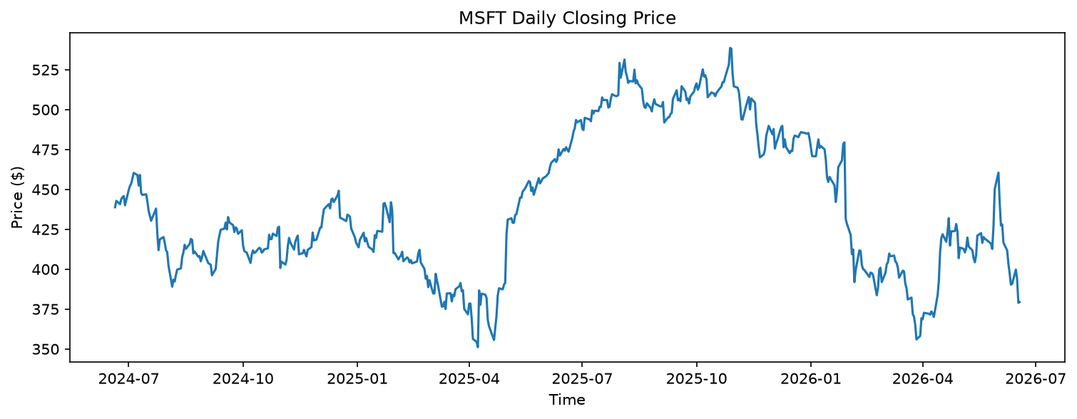
Now with some definitions and concepts made clearer, how can we actually test for whether or not a series is stationary? We can conduct what is called the Augmented Dickey-Fuller (ADF) test. What it is at the end of the day is it is a test of statistical significance, where we have our null and alternative hypotheses and will calculate a test statistic, p value, and make a decision as to whether the series is stationary or not. To better understand how this test works, we need to understand what a unit root is. Consider a simple AR(1) model, $x_t = b_1 x_{t-1} + \varepsilon_t$ . If the coefficient $b_1 = 1$ , the series has a unit root and is not stationary — this is precisely the random walk we just defined above ( $x_t = x_{t-1} + \varepsilon_t$ ). If $b_1 < 1$ , the series is stationary, since past shocks decay over time rather than persisting forever. The ADF test is an extension of the DF test that tests for this presence of a unit root, with the null hypothesis being that the series has a unit root, and the alternative hypothesis being that we do not ie the series is stationary. The decision rule is standard: if the p-value falls below a chosen significance level (typically 0.05), we reject the null and conclude the series is stationary; otherwise, we fail to reject, and treat the series as non-stationary. Let's test this on a real stock. Here's MSFT's daily closing price over the last two years:

import yfinance as yf
import matplotlib.pyplot as plt
from statsmodels.tsa.stattools import adfuller

data = yf.Ticker('MSFT').history(period="2y", interval="1d")
close_prices = data.loc[:, 'Close'].dropna()

plt.figure(figsize=(12,4))
plt.plot(close_prices)
plt.title('MSFT Daily Closing Price')
plt.xlabel('Time')
plt.ylabel('Price ($)')
plt.show()

result = adfuller(close_prices)
print(f"ADF Statistic: {result[0]:.4f}")
print(f"p-value: {result[1]:.4f}")

MSFT closing price

ADF Statistic: -1.4561
p-value: 0.5551

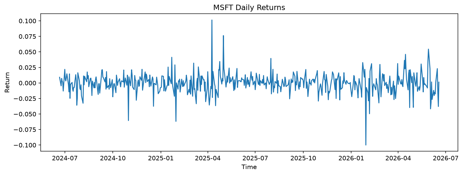
Running the ADF test on the raw price series, we'd expect a high p-value — well above 0.05 — meaning we fail to reject the null hypothesis. The price series behaves like a random walk: it wanders over time with no fixed mean to revert to. Now let's difference the series by converting prices into returns, and run the test again:

returns = close_prices.pct_change().dropna()

plt.figure(figsize=(12,4))
plt.plot(returns)
plt.title('MSFT Daily Returns')
plt.xlabel('Time')
plt.ylabel('Return')
plt.show()

result2 = adfuller(returns)
print(f"ADF Statistic: {result2[0]:.4f}")
print(f"p-value: {result2[1]:.4f}")

MSFT returns

ADF Statistic: -21.1794
p-value: 0.0000

Differencing once — turning the price series into a returns series — should collapse the p-value to near zero, letting us reject the null in favor of stationarity. This is the "d=1" step in ARIMA in action: differencing once is enough to turn a non-stationary, wandering price series into a stationary returns series.

ACF and PACF

Now that we understand what stationarity is and how to test for it, we need to be able to measure how much the time series depends on its past, also known as autocorrelation. Autocorrelation is defined as a series compared to a lagged version of itself. Recall that one of the conditions for weak stationarity is that the covariance between $x_t$ and $x_{t+k}$ depends only on the lag $k$ , not on $t$ itself. The Autocorrelation Function (ACF) will allows us to measure and see that relationship across every lag at once. PACF, on the other hand, answers a more specific question. It focuses on the direct correlation at each lag after removing the effect of every shorter lag. A good way to visualize the difference between the 2 is as follows. Say we are looking at intra-week data and are comparing the price of a stock on Monday vs Wednesday. And say we identify some correlation between the 2 days. When using ACF, that relationship captures the correlation of both Monday to Tuesday and Tuesday to Wednesday, whereas PACF isolates the Monday to Wednesday relationship once the other portion has been accounted for. Here's the ACF and PACF for MSFT's daily returns (the same series we made stationary in the ADF section above):

import matplotlib.pyplot as plt
from statsmodels.graphics.tsaplots import plot_acf, plot_pacf

fig, axes = plt.subplots(2, 1, figsize=(10, 6))
plot_acf(returns, lags=30, ax=axes[0])
axes[0].set_title('ACF of MSFT Daily Returns')
plot_pacf(returns, lags=30, ax=axes[1])
axes[1].set_title('PACF of MSFT Daily Returns')
plt.tight_layout()
plt.savefig('msft_acf_pacf.png', dpi=150, bbox_inches='tight')
plt.show()

MSFT acf/pacf

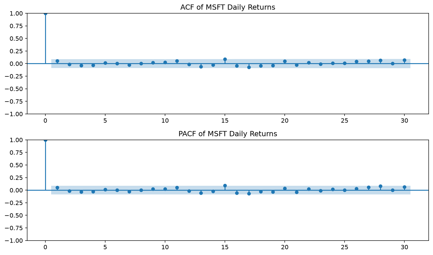
For a stock return series like the one above, it is expected for the lags represented in these plots to fall within the confidence band.

AR(p)

Building upon this idea of autoregression, the AR(p) model is the generalized form of the autoregressive model where the current value in the series depends on p past values. Being able to choose the correct p value is important. Too low, and the model can't capture the real dependency structure in the data. Too high, and you risk overfitting of the model, calculating inflated test statistics on in-sample data and making forecasts worse. This is where the PACF test comes into play. For an AR(p) process, the PACF cuts off sharply after lag p — the partial autocorrelations beyond that point should fall inside the confidence band — while the ACF tails off gradually. In practice, this means you can often read p directly off the PACF plot before fitting anything.

MA(q)

A Moving Average (MA) model is similar to an autoregressive model except that instead of being a lagged version of past values, it is a lagged version of past white noise values. This means that the MA model captures the white noise "shocks" directly at each current value of the model as opposed to indirectly through the AR model, but only for q periods, after which it has no effect at all. The pattern for of using acf/pacf is flipped for an MA(q) model. For an MA(q) model, the ACF cuts off sharply after lag q while the PACF tails off gradually.

The moment you've been waiting for: ARIMA(p,d,q)

We have now laid all of the groundwork and are ready to go through the ARIMA model. What it is is simply a combination of the AR and MA models, a series that can be modeled through a lagged version of itself and past shocks. The model also adds I, standing for integrated which just means the data is stationary. Now moving on to the parameters of the model, which were defined above but lets go ahead and clarify them in their own definitions:

p: number of autoregressive terms ie the number of lagged observations
d: the number of differencing, applied d times to turn a non-stationary series into a stationary one
q: number of lagged forecast error terms

In practice, you can find the p and q values directly from the ACF/PACF plots we created from earlier, identifying the lag where each plot's bars drop inside the confidence band. In reality, it is better to utilize some information criterion such as AIC or BIC. Since we are forecasting or "predicting" stock prices, we will use the AIC since the AIC penalizes unnecessary complexity while still rewarding fit, which matters when we'd rather not overfit a model that's trying to forecast prices.

from pmdarima import auto_arima

model = auto_arima(close_prices, start_p=0, start_q=0, max_p=5, max_q=5, d=1,
                    seasonal=False, trace=True, suppress_warnings=True)

Best model: ARIMA(0,1,0)

So with order (0,1,0) in hand, here's what the resulting forecast actually looks like:

import pandas as pd
from statsmodels.tsa.arima.model import ARIMA

model = ARIMA(close_prices, order=(0, 1, 0))
fit = model.fit()

forecast_result = fit.get_forecast(steps=30)
mean_forecast = forecast_result.predicted_mean
conf_int = forecast_result.conf_int(alpha=0.05)

# build a proper date index continuing from the last real date
last_date = close_prices.index[-1]
forecast_index = pd.bdate_range(start=last_date, periods=31)[1:]  # business days, skip day 0 (already have it)
mean_forecast.index = forecast_index
conf_int.index = forecast_index

plt.figure(figsize=(12,4))
plt.plot(close_prices[-100:], label='Actual')
plt.plot(mean_forecast, label='Forecast', color='tab:orange')
plt.fill_between(
    forecast_index,
    conf_int.iloc[:, 0],
    conf_int.iloc[:, 1],
    color='tab:orange',
    alpha=0.2,
    label='95% Confidence Interval'
)
plt.legend()
plt.title('MSFT ARIMA Forecast vs Actual')
plt.savefig('msft_arima_forecast.png', dpi=150, bbox_inches='tight')
plt.show()

MSFT arima forecast

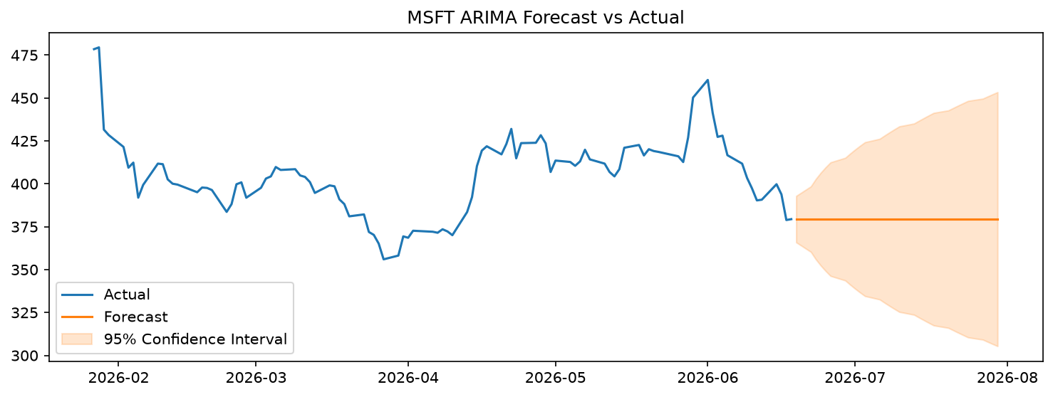
And... a mere flat line prediction?? This is indeed not a bug in our code, but rather an honest assessment of what this model is capable of based on our data. When using order (0,1,0) for our model, there is no AR or MA term to forecast any structure in our data, the best estimate for tomorrow's price is simply today's price. Even after observing substantial price movements in MSFT, the model's forecast will not extrapolate that movement because there is no statistical basis to do so. Notice, too, that the shaded band around the forecast grows wider the further out it projects — the model's single best guess never moves, but subsequent guesses are more and more distributed in their likely outcomes. If MSFT's returns truly behave like white noise, then no amount of searching for p and q values should find structure that isn't there, and that's exactly what auto_arima confirmed when it landed on (0,1,0).

Conclusion

After all that work, it can seem disappointing to conclude that ARIMA models are indeed not particularly useful in forecasting stock prices into the future. Where this model does hold useful application is in time series that exhibit actual autocorrelation, such as CPI data, trading volume, or even weather patterns. And I am definitely interested in using the ARIMA model more directly, such as through these type of series available on prediction markets, something worth exploring down the road. However, where I would like to go next is how we can apply these types of stock series to the idea of cointegration and pairs trading, which is what we will be exploring next.